Raymarching (not to be confused with ray tracing) is one of the most interesting ways to render voxels. It’s performant, parallelizes well, and doesn’t require much upfront computation. Of course it comes at a cost — it’s fragment shader heavy so you’ll like end up fillrate limited. Its complexity also makes it a tad fragile; a little floating point error buildup can cause tunneling and subtle artifacts.
For a little context, take a look at Inigo Quilez’s excellent work and writeups with ray marching. One caveat is that his work primarily focuses on signed distance fields, which the techniques below are not — unsigned distance fields are closer to being accurate.
So, on to the techniques. I’ll cover three primary techniques:
- Raymarching plane intersections. A set of NxNxN voxels can be divided up using N+ 1 planes along each axis. An easy approach to raymarching is to take a ray for each fragment and march it along each plane intersection until a non-empty voxel is found.
- Sphere assisted raymarching. This technique reduces the number of voxel lookups, though it’s not always a performance win. The basic idea is to store the shape information separate from the color information. Then, instead of storing the shape information directly, each empty voxel stores the radius of the empty space around it — representing the largest sphere that could fill the empty space centered a the current voxel. This allows for large steps through empty space.
- Cube assisted raymarching. Similar to the previous technique, except instead of the largest sphere, the shape information stores the largest cube possible around the current location. Why a cube instead of a sphere? Because it’s much much faster to compute — an order of magnitude faster. Its shape is slightly suboptimal, but still gets most of the speedup from the previous technique.
Test setup
Like in my previous tests, to compare these techniques I started by throwing a bunch of 32x32x32 voxel spheres at them and measuring the memory impact and per-frame render times. In addition, a degenerate case of a 32x32x32 voxel set with only a single solid voxel in its corner was added to demonstrate where the plane marching technique falls short.
The same test machine and setup was used — 1920x1080 on Windows 10 using a GTX 980 Ti, Intel i7–4790k, and 16GB of main memory.
I added an additional constraint that the previous tests didn’t have. All techniques must produce a pixel perfect match for their quad based brethren. This is important because it’s easy to cut a few corners and get a perf boost at the cost of accuracy — or to let floating point error cause close but incorrect results.
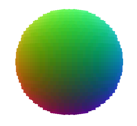 Figure 1. The voxel object used.
For each technique, the test is repeated for different numbers of objects to allow trends to emerge. The largest data set contains 16k voxel objects and is enough to strain the test system.
I posted the full source for these tests on GitHub. I encourage you take a look — a source file is worth a thousand words.
Raymarching Overview
Raymarching is an interesting rendering technique. It takes a ray consisting of an origin p0 and a direction d . It then checks points along the ray for being inside a solid object. To do this, it iteratively marches along the ray, starting at p0 and taking non-uniform steps along the ray. At each step, the distance to the closest possible intersection is conservatively estimated — it can be overestimated, but must never be underestimated — and a step of that size is then taken.
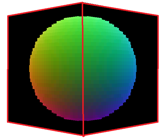 Figure 2. A raymarched voxel sphere rendered on the surface of a cube.
Raymarching requires a termination criteria. In the case of signed distance fields (a typical example Google will turn up), this criteria is convergence. Step sizes will eventually approach zero and the intersection will be determined to have been found. In our case, we can simplify things by checking if the current point is inside a solid voxel.
For rendering voxel objects, each object, no matter how many voxels it contains, is rendered using a cube. Six quads are sent into the render pipeline and the fragment shader does the hard work of finding the intersections by marching rays from the cube’s surface.
Putting this together in a fragment shader, it becomes:
vec4 March(vec3 p0, vec3 d) {
  float t = 0;
  while (t < someMaxDistToCheck) {
    vec3 p = p0 + d * t;
    if (IsVoxelSolid(p)) {
      return VoxelColor(p);
    }
    t += EstimateIntersectionDistance();
  }
  return vec4(0);
}
The important piece here is distance estimation function, which the specific techniques will fill in.
Raymarching Plane Intersections technique
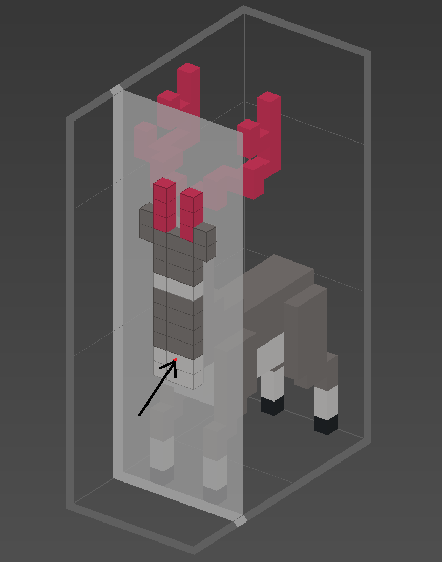 Figure 3. A voxel reindeer showing a single plane-ray intersection.
This technique imagines planes separating each layer of voxels. A ray is then marched along each plane intersection and the voxels at the intersection points are checked for being solid.
It’s important to check the the intersection points in the order in which the ray reaches them. The key here is that planes along all three axes will need to be checked each step, with the closest intersection being the step taken.
Working in voxel-unit-space (i.e. where one voxel is 1x1x1 units in size) finding these intersections becomes easy. Simply check the fraction require to round up to the next integer (or down for negative directions) and then divide by the appropriate component of d to make it exact. This works out to be:
vec4 PlaneMarch(vec3 p0, vec3 d) {
  float t = 0;
  while (t <= maxDistToCheck) {
    vec3 p = p0 + d * t;
    vec4 c = textureLod(voxels, p / voxelGridSize, 0);
    if (c.a > 0) {
      return c;
    }

    vec3 deltas = (step(0, d) - fract(p)) / d;
    t += max(mincomp(deltas), epsilon);
  }

  return vec4(0);
}
Notice there’s a tiny epsilon to guarantee there’s always at least a small amount of progress.
This technique works well, but notice how it will never move more than a single voxel at a time. Wouldn’t it be nice to skip over all of those empty voxels we check before reaching a solid one? Well, we can — at least some of them.
Sphere Assisted Raymarching
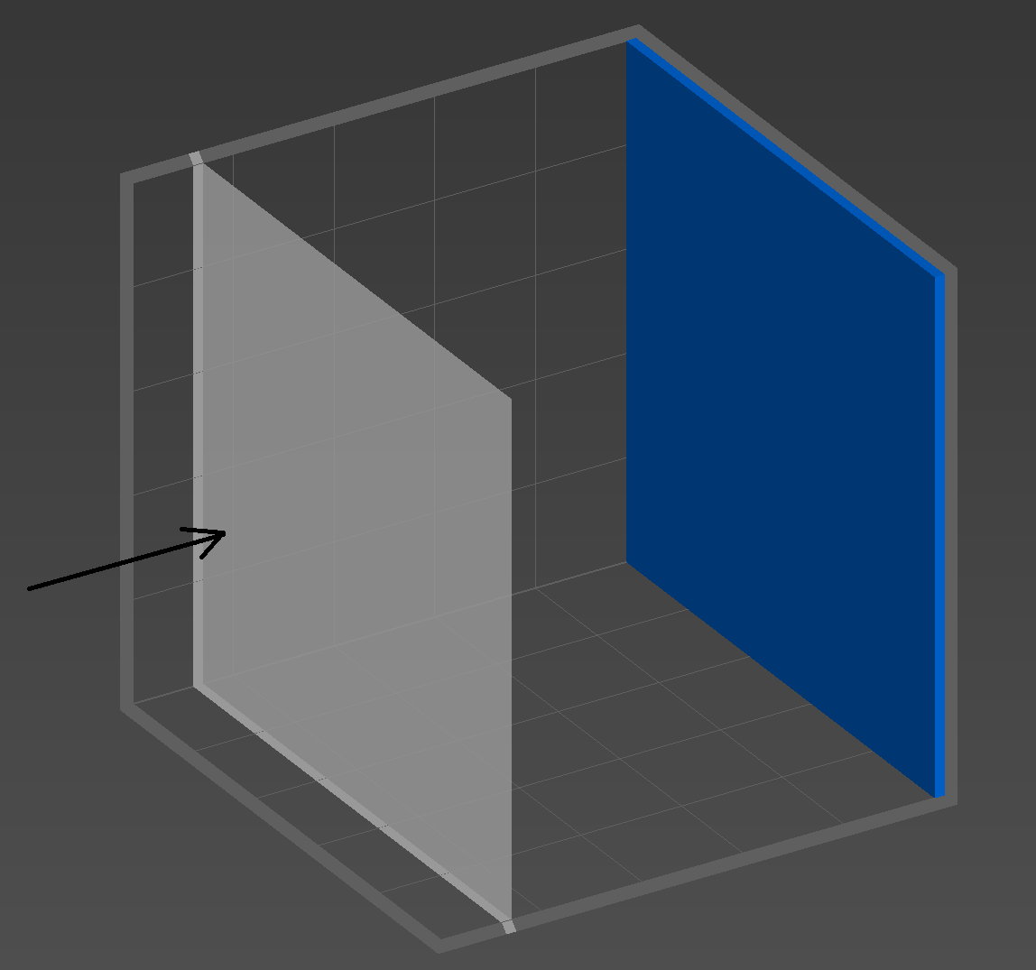 Figure 4. Degenerate case for the previous technique — lots of checking of empty voxels.
In the previous technique, all voxel information was crammed in a single 3D texture, with the alpha channel giving information about whether or not the voxel is solid. This is straightforward and works well — especially since only a single texture needs to be swapped between objects. However, some degenerate cases will require many steps checking empty voxels.
The worst case scenario for the previous technique is, rather ironically, an empty set of voxels. Each ray will have to pass through the entire object before deciding there’s nothing to hit and terminating. A less trivial case would be a voxel object with only a wall of solid voxels at the far end of the z-axis. Viewed with the wall on the far side, each ray will have to traverse the entire width of the object before finding its destination — obviously not ideal. Figure 4 shows this case.
Enter sphere assisted raymarching to help. Instead of storing simply solid/not solid values in the alpha channel, we can store the distance to the nearest solid voxel. Then, when traversing an empty voxel, we can take a massive step across many empty voxels. Pretty neat, huh?
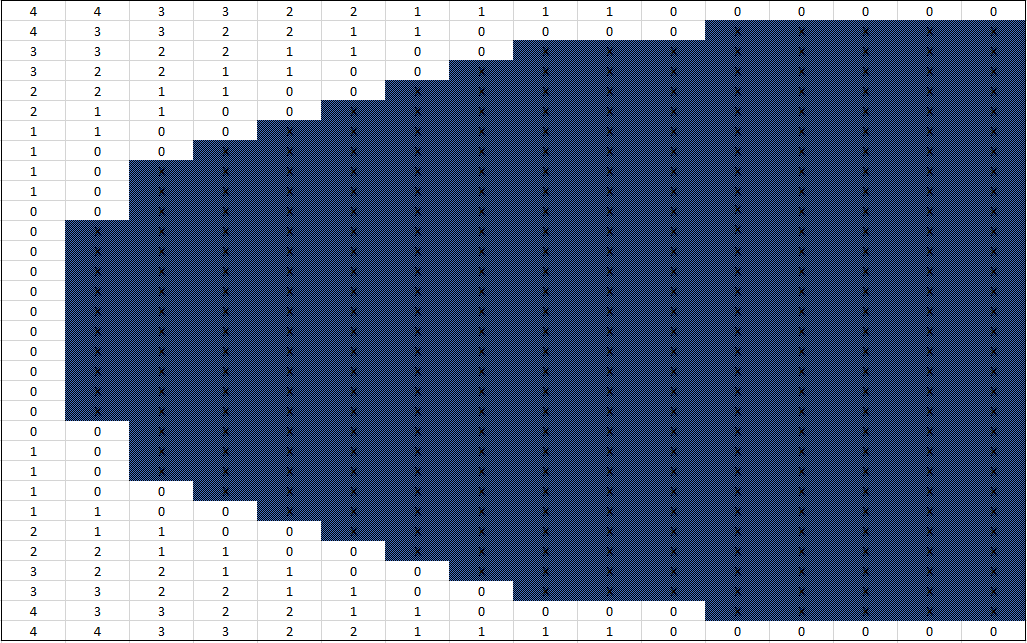
Figure 5 is a cross section of what such a technique would generate. The blue cells represent the solid voxels. The white cells are empty, and store the amount of distance that can be safely moved before reaching a solid voxel.
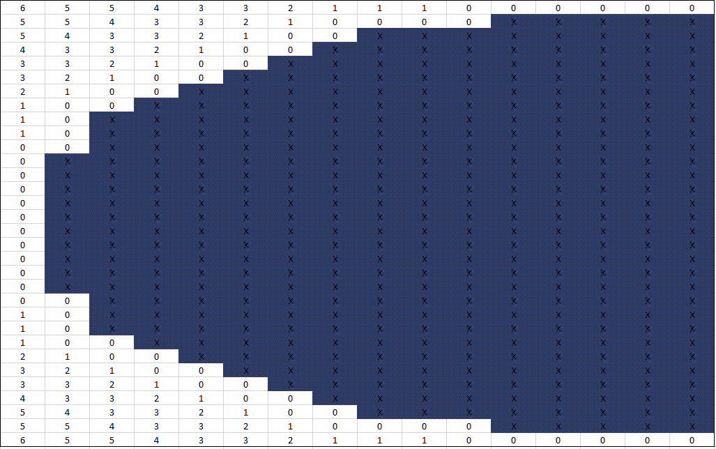 Figure 5. A cross section of a sphere-assisted shape.
The hard part is generating this shape data. It’s important to notice that we’ve gone from normalized floating point values for the shape data to non-negative integers. To keep using normalized floats for the color channels, the shape data is split off into an integer 3D texture.
The changes needed for the fragment shader are pretty minimal:
vec4 ShapeMarch(vec3 p0, vec3 d) {
  float t = 0;
  while (t <= maxDistToCheck) {
    vec3 p = p0 + d * t;
    uint shapeValue = textureLod(shape, p / voxelGridSize, 0).r;
    if (shapeValue == 255) {
      return textureLod(voxels, p / voxelGridSize, 0);
    }

    vec3 deltas = (step(0, d) - fract(p)) / d;
    t += max(mincomp(deltas) + shapeValue, epsilon);
  }

  return vec4(0);
}
Shape assisted raymarching. 255 is a constant representing a solid voxel.
Cube Assisted Raymarching
The biggest drawback of sphere assisted raymarching is the upfront workload. A simple implementation runs in O(n²) time, with n being the number of voxels. This gets big fast — up to ~1,000,000 steps for a simple 32x32x32 voxel set. Enter cubes to save the day.
Similar to the sphere assisted raymarching, cube assisted raymarching checks how large of an object can be inserted around each empty cell; using cubes of course rather than spheres. This is slightly suboptimal in most cases, takes us from O(n²) upfront cost to O(n log n). How? Using a summed area table and a binary search for the right cube size.
Summed area tables are a neat data structure often seen in computer vision. A full explanation is beyond the scope of this article, but the executive summary is that they store the sum of all prior cells at a specific location. Using this information, it’s quick to compute the area of an arbitrary box by subtracting off the parts we’re not interested in. Once created, the area of an arbitrary box can be computed in O(1) time.
The algorithm for this is to (1) compute the summed area table and then (2) for each cell, binary search up to the maximum sized cube. Since area calculations using the table are O(1), each voxel takes only O(log n) time.
Comparing the resulting shape to the previous, we can see it’s not as efficient, though it’s still pretty good:
With our techniques in place, it’s time for some results.
Results
Render Time Results
The standard test set shows plane marching with a moderate lead over both shape assisted techniques. On the low end, render times are very close. However, as the set size increases, plane marching takes a pretty clear lead.
Time per frame (ms) — standard test case.
| Objects (k) | Plane Marching | Sphere Assisted | Cube Assisted |
|---|---|---|---|
| 1 | 1.2 | 0.8 | 0.8 |
| 2 | 6.9 | 4.4 | 4.8 |
| 3 | 2.6 | 3.2 | 3.1 |
| 4 | 5.6 | 4.2 | 4.2 |
| 5 | 3.6 | 5.3 | 5.2 |
| 6 | 7.0 | 6.3 | 6.5 |
| 7 | 4.3 | 7.3 | 7.4 |
| 8 | 7.9 | 8.3 | 8.5 |
| 9 | 5.2 | 9.5 | 9.5 |
| 10 | 8.5 | 10.5 | 10.4 |
| 11 | 6.6 | 11.3 | 11.3 |
| 12 | 8.2 | 12.4 | 12.0 |
| 13 | 8.0 | 13.5 | 13.1 |
| 14 | 8.1 | 14.2 | 14.6 |
| 15 | 8.6 | 15.5 | 15.2 |
| 16 | 9.3 | 16.8 | 16.2 |
Notice that how the performance hit for growing set sizes isn’t stable. This shows how our performance is both data and view dependent. The further the rays need to march into the object, the worse performance will be; one set of benchmarks can’t tell the whole story.
To get a better idea of what’s going on, I also benchmarked a degenerate case — a single solid voxel in the far corner of a 32x32x32 voxel set. This example is a bit contrived since the ideal thing to do here would be to shrink the set to 1x1x1 but it illustrates a general problem. Notice how vastly different the results are in the figure below for plane marching.
Time per frame (ms) — degenerate case.
| Objects (k) | Plane Marching | Sphere Assisted | Cube Assisted |
|---|---|---|---|
| 1 | 5.83 | 0.87 | 0.87 |
| 2 | 11.37 | 1.86 | 2.00 |
| 3 | 18.35 | 3.04 | 3.02 |
| 4 | 23.98 | 4.22 | 4.20 |
| 5 | 31.31 | 5.33 | 5.28 |
| 6 | 35.91 | 6.34 | 6.50 |
| 7 | 44.67 | 7.34 | 7.30 |
| 8 | 53.92 | 8.51 | 8.57 |
| 9 | 57.98 | 9.45 | 9.66 |
| 10 | 57.94 | 10.75 | 10.83 |
| 11 | 64.50 | 11.70 | 11.52 |
| 12 | 67.27 | 12.94 | 12.51 |
| 13 | 68.11 | 13.34 | 13.56 |
| 14 | 71.39 | 14.91 | 14.49 |
| 15 | 78.19 | 15.36 | 15.55 |
| 16 | 78.02 | 16.52 | 16.68 |
Both of the shape assisted techniques remain relatively the same with good performance.
Memory Impact
Although not as taxing as other techniques when it comes to memory (particularly VAOs and display lists), raymarching isn’t the most compact technique.
GPU memory used (MB).
| Objects (k) | Plane Marching | Sphere Assisted | Cube Assisted |
|---|---|---|---|
| 1 | 141.0 | 207.5 | 207.4 |
| 2 | 259.5 | 390.0 | 390.0 |
| 3 | 387.7 | 582.0 | 582.1 |
| 4 | 516.0 | 775.3 | 775.2 |
| 5 | 644.3 | 967.2 | 967.3 |
| 6 | 772.1 | 1159.3 | 1159.2 |
| 7 | 900.3 | 1351.2 | 1351.3 |
| 8 | 1019.6 | 1545.2 | 1545.1 |
| 9 | 1156.0 | 1735.2 | 1744.0 |
| 10 | 1285.3 | 1927.3 | 1927.2 |
| 11 | 1412.0 | 2119.2 | 2119.5 |
| 12 | 1541.3 | 2311.5 | 2311.1 |
| 13 | 1668.0 | 2505.0 | 2505.2 |
| 14 | 1797.3 | 2695.3 | 2695.2 |
| 15 | 1925.2 | 2889.1 | 2889.2 |
| 16 | 2055.2 | 3084.2 | 3084.1 |
To perform easy efficient raymarching, the entire voxel set for each object needs to be loaded into memory. This is in contrast with quad based techniques which only require data for solid voxels.
The one advantage raymarching has when it comes to memory is that it’s not data dependent. Any set of 32x32x32 voxels will take the same amount of memory regardless of their contents. Polygonal techniques will depend entirely on the data inside them, though they’re typically smaller.
Main memory usage is negligible, as is to be expected with nearly all of the work taking place on the GPU:
Main memory used (MB).
| Objects (k) | Plane Marching | Sphere Assisted | Cube Assisted |
|---|---|---|---|
| 1 | 10.9 | 10.5 | 11.4 |
| 2 | 24.4 | 34.1 | 34.5 |
| 3 | 29.3 | 44.0 | 42.9 |
| 4 | 37.9 | 55.7 | 56.7 |
| 5 | 39.7 | 66.7 | 62.2 |
| 6 | 47.7 | 76.9 | 78.1 |
| 7 | 51.1 | 83.6 | 83.0 |
| 8 | 69.1 | 102.2 | 104.9 |
| 9 | 61.8 | 106.2 | 97.7 |
| 10 | 70.8 | 124.7 | 120.1 |
| 11 | 75.9 | 123.8 | 123.7 |
| 12 | 80.1 | 139.2 | 147.0 |
| 13 | 84.0 | 150.2 | 148.2 |
| 14 | 92.3 | 157.1 | 157.3 |
| 15 | 95.4 | 167.2 | 177.8 |
| 16 | 106.4 | 199.9 | 187.5 |
Where to go from Here
Cube assisted raymarching seems like the way to go. It has a low upfront cost and performs well even in the worst case.
Looking towards the future, there are three particularly notable caveats:
- There are likely many performance gains to be had, so don’t take these render times to be absolute. Optimizing raymarching while maintaining accurate results is difficult — many potentially large optimizations were abandoned due to their numerical instability.
- Performance will be architecture dependent. I regret not having more platforms to benchmark as performance is likely to degrade quickly on both competing and older architectures.
- Lighting is going to be more complicated. With polygonal techniques, a normal can be passed down the pipeline cheaply. With raymarching, normals are generally found numerically by taking multiple samples, which could end up being costly and may create lighting artifacts.
Of course there’s also flexibility in raymarching. The techniques here can be easily combined with other ones such as rounded cubes or union/subtraction/intersection. It’ll also be a boon when voxel resolution is greater than render resolution.
3D hashing is a promising area thread to pull on to reduce memory overhead. For many voxel objects, only a small amount of colors will be used (compared to the size of the raw data set). By finding the final color after raymarching terminates via 3D hashing, a considerable amount of memory could be saved and the performance impact would likely be small — the bulk of the computation would still be the raymarching.
That’s it. Like last time, be sure to poke around with the code on GitHub:
cleak/VoxelPerf — Performance testing sandbox for voxel graphics